This is the 10th in a series of class notes as I go through the Georgia Tech/Udacity Machine Learning course. The class textbook is Machine Learning by Tom Mitchell.

This chapter is less theoretical than VC Dimensions, but still more focusing on the theoretical basis of what we do in Supervised Learning.

The Core Question

What we've been trying to do is: learn the best hypothesis that we can, given some data and domain knowledge.

We are going to refine what our notion of "best" is to be "most probable" hypothesis, out of the hypothesis space.

Bayes Rule

I'll assume you know this (more info, wonderful counterintuitive application here):

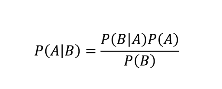
Applied to ML:

• A is our hypothesis
• B is our Data
• our hypothesis given the data is P(A|B), what we want to maximize
• our data sampling is P(B)
• our prior domain knowledge is represented by P(A)
• our updating (the running of the algorithm) is P(B|A), also considered accuracy

Since P(B) is constant among hypotheses and we just care about maximizing P(A|B), we can effectively ignore it.

We've had many ways of representing domain knowledge so far - SVM kernels, choosing to use kNN (closer is more similar) - P(A) is a more general form of this.

Maximum Likelihood: In fact if we further assume we have no priors (aka assume a uniform distribution for P(A)), P(A) can effectively be ignored. This means maximizing P(A|B) (our most likely hypothesis given data) is the same as maximizing P(B|A) (the most likely data labels we see given our hypothesis) if we don't have a strong prior. This is the philosophical justification for making projections based on data, but as you can see, even a little bit of domain knowledge will skew/improve our conclusions dramatically.

However, it is impractical to iterate through all hypotheses and mechanically update priors like this. What we are aiming for with Bayes is more of an intuition about the levers we can pull rather than an actual applicable formula.

The Relationship of Bayes and Version Spaces

No Noise: This proof is too mundane to write out, but basically given no priors, it is a truism that the probability of any particular hypothesis given data (P(h|D)) is exactly equal to 1/|VS| (VS for version space). AKA if all hypotheses are equally likely to be true, then the probability of any one hypothesis being true is 1 / the number of hypotheses. Not exactly exciting stuff, but it derives from Bayes.

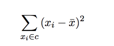
With Noise: If we assume that noise has a normal distribution, we then use this proof to arrive at the sum of squares best fit formula:

The Minimum Description Objective

By adding a logarithm (a monotonic function, so it doesnt change the end result), we can translate, decompose, and flip the maximization goal we defined above to a minimization with tradeoffs:

Here L stands for Length, for example the length of a decision tree, which indicates the complexity of the model/hypothesis. L(h) is the complexity of the model we have selected, while L(D|h) is the data that doesn't fit the model we have selected, aka the error. We want to minimize this total "description length", aka seek the minimum description length. This is a very nice mathematical expression of Occam's razor with a penalty for oversimplification.

There are practical issues with applying this, for example the unit comparability of errors vs model complexity, but you can decide on a rule for trading them off.

The Big Misdirection

Despite everything we laid out here and in prior chapters, we don't -really- care about finding the single best or most likely hypothesis. We care about finding the single most likely label. A correct hypothesis will help us get there every time, sure, but if every remaining hypothesis in our version spaces in aggregate point towards a particular label, then that is the one we actually want.

Thus, Bayesian Learning is merely a stepping stone towards Bayesian Classification, and building a Bayes Optimal Classifier.

We will explore this in the next chapter on Bayesian Inference.

Next in our series

Further notes on this topic:

• a nice introduction to Bayesian Learning with more detail
• application to neural networks, aka Bayesian Networks
• great discussion of Bayesian nonparametric learning

Hopefully that was a good introduction to Bayesian Learning. I am planning more primers and would love your feedback and questions on:

• Overview
• Supervised Learning
  • Decision Trees
  • Regression
  • Neural Networks
  • Instance Based Learning (K Nearest Neighbors)
  • Ensemble Learning (AdaBoost)
  • Kernel Methods & SVMs
  • Computational Learning Theory
  • VC Dimensions
  • Bayesian Learning
  • Bayesian Inference
• Unsupervised Learning
  • Randomized Optimization
  • Information Theory
  • Clustering - week of Feb 25
  • Feature Selection - week of Mar 4
  • Feature Transformation - week of Mar 11
• Reinforcement Learning
  • Markov Decision Processes - week of Mar 25
  • "True" RL - week of Apr 1
  • Game Theory - week of Apr 15