Welcome to this week’s tips and tricks blog where we explore both beginner and advanced YugabyteDB topics for PostgreSQL and Oracle DBAs. First things first, for those of you who might be new to either distributed SQL or YugabyteDB read on.
What is Distributed SQL?
Distributed SQL databases are becoming popular with organizations interested in moving data infrastructure to the cloud or to cloud native environments. This is often motivated by the desire to reduce TCO or move away from the scaling limitations of monolithic RDBMS like Oracle, MySQL and SQL Server. The basic characteristics of Distributed SQL are:
- A SQL API for querying and modeling data, with support for traditional RDBMS features like primary keys, foregin keys, indexes, stored procedures, and triggers.
- Automatic distributed query execution so that no single node becomes a bottleneck.
- A distributed SQL database should support automatically distributed data storage. This includes indexes which should be automatically distributed (aka sharded) across multiple nodes of the cluster so that no single node becomes a bottleneck for ensuring high performance and high availability.
- Distributed SQL systems should also provide for strongly consistent replication and distributed ACID transactions. For a deeper discussion about what Distributed SQL is, check out, “What is Distributed SQL?”
What is YugabyteDB?
YugabyteDB is an open source, high-performance distributed SQL database built on a scalable and fault-tolerant design inspired by Google Spanner. YugabyteDB is PostgreSQL wire compatible with support for advanced RDBMS features like stored procedures, triggers, and UDFs.
Got questions? Make sure to ask them in our YugabyteDB Slack channel. Please note that most examples in the post make use of the Northwind sample database. Instructions on how to get it installed are here.
Ok, let’s dive in…
Is there a functional equivalent to Oracle’s NVL in PostgreSQL or YugabyteDB?
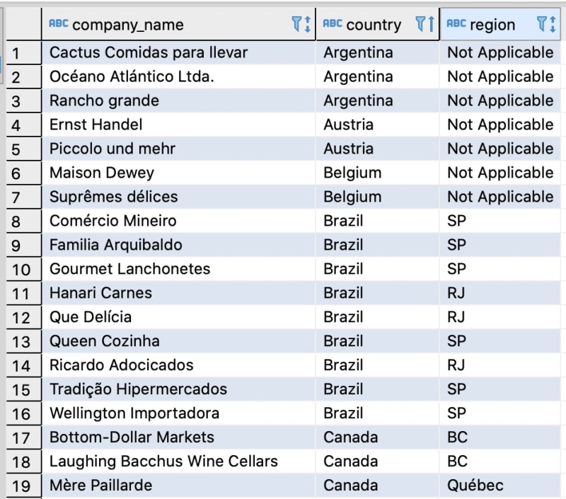
In a nutshell, Oracle’s NVL lets you replace NULL, which returns as a blank in the results of a query with a string. For example, let’s say we want to return a list of our customers and for those that have NULL in the region column, swap in “Not Applicable.”
SELECT company_name, country, NVL(region, 'Not Applicable')
FROM customers
ORDER BY country;
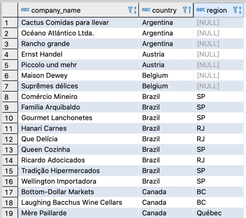
To achieve similar results in PostgreSQL and YugabyteDB, we can use the COALESCE function. So, to start, here’s the partial output of our customers table. Note that Argentina, Austria and Belgium have NULL in the region column.
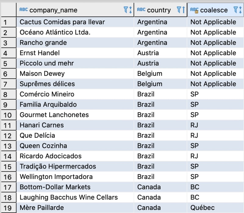
With the COALESCE function we can make the swap.
SELECT company_name, country, COALESCE (region, 'Not Applicable')
FROM customers
ORDER BY country;
Does YugabyteDB support PostgreSQL’s Views, Materialized Views, and Rollups?
VIEW and ROLLUP are supported, with materialized view support currently in development. You can track its development with this GitHub issue.
PostgreSQL’s views can be thought of as “virtual tables” that bring together data from one or more tables that can be queried against, just like a regular table. A materialized view on the other hand is not “virtual,” so we don’t have to recompute the view every time we want to access it. This makes materialized views much more efficient to query, with the trade offs of requiring additional storage and when there are updates to the base tables of the view, the materialized view must also be kept updated.
Finally, PostgreSQL’s ROLLUP is a subclause of GROUP BY that allows us to define multiple grouping sets. This is especially useful in analytic use cases where you might want to “rollup” dates, monetary values or other types of data where some calculation might be useful. Let’s walk through each example.
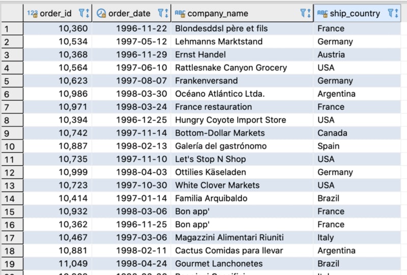
Creating a VIEW in YugabyteDB is identical to how it is done in PostgreSQL. In this example, let’s create a VIEW on the customers and orders table. In this scenario a VIEW is useful because although the customer_id column exists in both the orders and customers tables, company_name does not exist in the orders table. We want to make it super simple to get the order details and customer_name associated with the order in one shot.
CREATE VIEW orders_by_company_name AS
SELECT orders.order_id, orders.order_date, customers.company_name, orders.ship_country
FROM orders, customers
WHERE orders.customer_id = customers.customer_id;
Now issue a simple SELECT statement to retrieve just the data that we need.
SELECT * FROM orders_by_company_name;
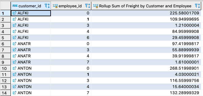
Creating a ROLLUP in YugabyteDB is identical to how it is done in PostgreSQL. For example, let’s say we want to “rollup” the data in our orders table so that the data is grouped by customer_id (who placed the order), employee_id (who took the order), and the total sum of freight sent.
SELECT
customer_id,
COALESCE(employee_id, '0') as employee_id,
    SUM (freight) as "Rollup Sum of Freight by Customer and Employee"
FROM
    orders
GROUP BY
    ROLLUP (customer_id, employee_id)
ORDER BY customer_id, employee_id;
From the output above we can see that the result set sums the freight by customer_id and employee_id.
Does YugabyteDB support EXPLAIN ANALYZE?
Yes. PostgreSQL’s EXPLAIN is a useful tool for determining where potential performance tuning opportunities lie with queries being issued against the database. Adding the ANALYZE option causes the statement to be actually executed, not only planned.
Let’s issue a simple EXPLAIN ANALYZE against the orders table in the northwind sample database. In this example we are executing queries against a YugabyteDB cluster with a replication factor of 3.
EXPLAIN ANALYZE SELECT customer_id, order_id, ship_country
FROM orders
WHERE order_date BETWEEN '1997-01-01' and '1999-12-31';

QUERY PLAN
----------
Foreign Scan on orders
(cost=0.00..105.00 rows=1000 width=82)
(actual time=4.865..27.046 rows=678 loops=1)

Filter: ((order_date >= '1997-01-01'::date) AND (order_date <= '1999-12-31'::date)

Rows Removed by Filter: 152
Planning Time: 31.899 ms
Execution Time: 29.078 ms
Next, let’s build an index on the order_date column and see if we can’t shave some time off the query.
CREATE INDEX idx_order_date
ON orders(order_date ASC);
We execute the same query and get the following results.
QUERY PLAN
----------
Index Scan using idx_order_date on orders
(cost=0.00..5.25 rows=10 width=82)
(actual time=10.350..11.607 rows=678 loops=1)

Index Cond: ((order_date >= '1997-01-01'::date) AND (order_date <= '1999-12-31'::date))
Planning Time: 13.608 ms                                                                                                   Execution Time: 11.913 ms
As you can see we are now able to confirm that by creating the index on the order_date column we were able to make an improvement on our planning time and execution time. The delta in the example is not dramatic, but you get the idea. With more complex queries and larger datasets, EXPLAIN and ANALYZE become essential performance tuning tools.

